Brownian motion¶

Preparing For This Tutorial:¶

Preparing For This Tutorial:

• The Robot that coincides with this tutorial comes from building specific sections found in the LEGO® MINDSTORMS® Education-Core set.

• You will need to build the main body for the robot (I’ll refer to use the Driving Base), plus a gyro sensor.

Exercises¶

1. Implement a program, using Python code, that using a random sequence of a fixed number of iterations makes the robot move along a straight line, and determine the average distance from the initial position. On the contrary, write a random walk program that allows the robot to reach a certain point along a straight line and determine the average value of the necessary steps.

2. Implement a program, using Python code, that using a random sequence of a fixed numbers of iterations makes the robot move along a broken line in the plain, and determine the average distance from the initial position, increase the number of steps, change the robot speed and the average path between to virtual collisions.

Theory¶

Brownian motion is the random movement of particles in a fluid due to their collisions with other atoms or molecules. Brownian motion is also known as pedesis, which comes from the Greek word for “leaping.” Even though a particle may be large compared to the size of atoms and molecules in the surrounding medium, it can be moved by the impact with many tiny, fast-moving masses. Brownian motion may be considered a macroscopic (visible) picture of a particle influenced by many microscopic random effects.

The one-dimensional random walk

The random walk is central to statistical physics. It is essential in predicting how fast one gas will diffuse into another, how fast heat will spread in a solid, how big fluctuations in pressure will be in a small container, and many other statistical phenomena.

The Probability of Landing at a Particular Place after n Steps

Let’s begin with walks of a few steps, each of unit length, and look for a pattern. We define the probability function f_N(n) as the probability that in a walk of N steps of unit length, randomly forward or backward along the line, beginning at 0, we end at point n. Since we have to end up somewhere, the sum of these probabilities over n must equal 1. We will only list nonzero probabilities. For a walk of n₀ steps, f0(0)=1. For a walk of one step, f1(−1)=1/2,  f1(1)=1/2. For a walk of two steps, f2(−2)=1/4,  f2(0)=1/2,  f2(2)=1/4. It is perhaps helpful in figuring the probabilities to enumerate the coin flip sequences leading to a particular spot. For a three-step walk, HHH will land at 3, HHT, HTH and THH will land at 1, and for the negative numbers just reverse H and T. There are a total of 23 = 8 different three-step walks, so the probabilities of the different landing spots are: f₃(−3)=1/8 (just one walk), f₃(−1)=3/8(three possible walks), f3(1)=3/8,  f3(3)=1/8.

For a four-step walk, each configuration of H’s and T’s has a probability of (1/2)4=1/16.

So f₄(4)=1/16, since only one walk—HHHH— gets us there.f₄(2)=1/4, four different walks, HHHT, HHTH, HTHH and THHH, end at 2. f₄(0)=3/8, from HHTT, HTHT, THHT, THTH, TTHH and HTTH.

Probabilities and Pascal’s Triangle

If we factor out the 1/2N, there is a pattern in these probabilities:

This is Pascal’s Triangle

every entry is the sum of the two diagonally above. These numbers are in fact the coefficients that appear in the binomial expansion of (a+b)N.

For example, the row for 25f5(n)

mirrors the binomial coefficients:

\({(a + b)}^{5} = a^{5} + 5a^{4}b + 10a^{3}b^{2} + 10a^{2}b^{3} + 5ab^{4} + b^{5}\)

To see how these binomial coefficients relate to our random walk, we write:

\({(a + b)}^{5} = (a + b) \cdot (a + b) \cdot (a + b) \cdot (a + b) \cdot (a + b)\)

and think of it as the sum of all products that can be written by choosing one term from each bracket. There are 25 = 32 such terms (choosing one of two from each of the five brackets), so the coefficient of \(a^{3}b^{2}\) must be the number of these 32 terms which have just 3 a’s and 2 b’s.

But that is the same as the number of different sequences that can be written by rearranging HHHTT, so it is clear that the random walk probabilities and the binomial coefficients are the same sets of numbers (except that the probabilities must of course be divided by 32 so that they add up to one).

Finding the Probabilities Using the Factorial Function

The efficient way to calculate these coefficients is to use the factorial function. Suppose we have five distinct objects, A, B, C, D, E. How many different sequences can we find: ABCDE, ABDCE, BDCAE, etc.? Well, the first member of the sequence could be any of the five. The next is one of the remaining four, etc. So, the total number of different sequences is 5×4×3×2×1 which is called “five factorial” and written 5! But how many different sequences can we make with HHHTT? In other words, if we wrote down all 5! (that’s 120) of them, how many would really be different? Since the two T’s are identical, we wouldn’t be able to tell apart sequences in which they had been switched, so that cuts us down from 120 sequences to 60. But the three H’s are also identical, and if they’d been different there would have been 3! = 6 different ways of arranging them. Since they are identical, all six ways come out the same, so we have to divide the 60 by 6, giving only 10 different sequences of 3 H’s and 2 T’s. This same argument works for any number of H’s and T’s. The total number of different sequences of m H’s and n(T)’s is (m+n)!/(m!n!) the two factorials in the denominator coming from the fact that rearranging the H’s among themselves, and the T’s among themselves, gives back the same sequence. It is also worth mentioning that in the five-step walk ending at –1, which has probability 10/25, the fourth step must have been either at 0 or –2. Glancing at Pascal’s Triangle, we see that the probability of a four-step walk ending at 0 is 6/24, and of ending at –2 is 4/24. In either case, the probability of the next step being to –1 is ½, so the total probability of reaching –1 in five steps is ½×6/24 + ½ ×4/24. So the property of Pascal’s triangle that every entry is the sum of the two diagonally above is consistent with our probabilities.

Probability Distribution

Let’s now consider a longer walk. After N= 100 steps, what is the probability of landing on the integer n ? This will happen if the number of forward steps exceeds the number of backward steps by n (which could be a negative number). That is,

nforward−nbackward=n

nforward+nbackward= N =100

from which

nforward=1/2(100+n), nbackward=1/2(100−n).

Note that in the general case, if the total number of steps N is even, nforward, nbackwardare both even or both odd, so n,the difference between them, is even, and similarly odd N means odd n. The total number of paths ending at the particular point n, from the heads and tails argument above, is

100!(nforward)!(nbackward)!=100!(1/2(100+n))!(1/2(100−n))!.

To find the actual probability of ending at n after 100 steps, we need to know what fraction of all possible paths end at n. (Since the coin toss is purely random, we take it that all possible paths are equally likely). The total number of possible 100-step walks is 2100≅1.26×1030.We’ve used Excel to plot the ratio: (number of paths ending at n)/(total number of paths) for paths of 100 random steps. The actual probability of landing back at the origin turns out to be about 8%, as is (approximately) the probability of landing two steps to the left or right. The probability of landing at most ten steps from the beginning is better than 70%, that of landing more than twenty steps away well below 5%.

(Note: It’s easy to make the graph yourself using Excel. Just write -100 in A1, then =A1 + 2 in A2, then =(FACT(100))/(FACT(50 - A1/2)*FACT(50+A1/2))*2^-100 in B1, dragging to copy these formulae down to row 101. Then highlight the two columns, click ChartWizard, etc.)

It is also worth plotting this logarithmically, to get a clearer idea of how the probabilities are dropping off well away from the center. This looks a lot like a parabola and it Well, to be precise, the logarithm of the probability distribution tends to a parabola as N becomes large, provided n is much less than N, and in fact this is the important limit in statistical physics. The natural log of the probability of ending the path at n tends to lnC−n2/200,where the constant Cis the probability (100!/50!50!)/2100 of ending the path exactly where it began. This means that the probability P(n) itself is given by:

P(n)=Ce−n2200, C≅0.08.

This is called a Gaussian probability distribution. The important thing to notice is how rapidly it drops once the distance from the center of the distribution exceeds 10 or so. Dropping one vertical space is a factor of 100!

So, How Far Away Should You Expect to Finish?

Since forward and backward steps are equally likely at all times, the expected average finishing position must be back at the origin. The interesting question is how far away from the origin, on average, we can expect to land, regardless of direction. To get rid of the direction, we compute the expected value of the square of the landing distance from the origin, the “mean square” distance:

E_n(d) = (2n/π)^(1/2)

Where every single step is considered of unit length.

After 100 steps, it should be at the distance of 8 units from the starting points ( the origin).

Two-dimensional random walk

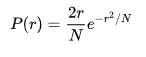
In higher dimensions, the set of randomly walked points has interesting geometric properties. In fact, one gets a discrete fractal, that is, a set which exhibits stochastic self-similarity on large scales. On small scales, one can observe “jaggedness” resulting from the grid on which the walk is performed. The trajectory of a random walk is the collection of points visited, considered as a set with disregard to when the walk arrived at the point. In one dimension, the trajectory is simply all points between the minimum height and the maximum height the walk achieved. To visualize the two-dimensional case, one can imagine a person walking randomly around a city. At every intersection, the person randomly chooses one of the possible routes (including the one originally travelled from). Formally, this is a random walk on the set of all points in the plane with. The asymptotic function for a two-dimensional random walk as the number of steps increases is given by a Rayleigh distribution. The probability distribution is a function of the radius from the origin and the step length is constant for each step:

Relation to Wiener process

Simulated steps approximating a Wiener process in two dimensions

A Wiener process is a stochastic process with similar behavior to Brownian motion, the physical phenomenon of a minute particle diffusing in a fluid. (Sometimes the Wiener process is called “Brownian motion”, although this is strictly speaking a confusion of a model with the phenomenon being modeled.)

A Wiener process is the scaling limit of random walk in dimension 1. This means that if you take a random walk with very small steps, you get an approximation to a Wiener process (and, less accurately, to Brownian motion). To be more precise, if the step size is ε, one needs to take a walk of length L/ε2 to approximate a Wiener length of L. As the step size tends to 0 (and the number of steps increases proportionally), random walk converges to a Wiener process in an appropriate sense. Formally, if B is the space of all paths of length L with the maximum topology, and if M is the space of measure over B with the norm topology, then the convergence is in the space M. Similarly, a Wiener process in several dimensions is the scaling limit of random walk in the same number of dimensions.

A random walk is a discrete fractal (a function with integer dimensions; 1, 2, …), but a Wiener process trajectory is a true fractal, and there is a connection between the two. For example, take a random walk until it hits a circle of radius r times the step length. The average number of steps it performs is r2. This fact is the discrete version of the fact that a Wiener process walk is a fractal of Hausdorff dimension. In two dimensions, the average number of points the same random walk has on the boundary of its trajectory is r4/3. This corresponds to the fact that the boundary of the trajectory of a Wiener process is a fractal of dimension 4/3, a fact predicted by Mandelbrot using simulations. A Wiener process enjoys many symmetries; random walk does not. For example, a Wiener process walk is invariant to rotations, but the random walk is not, since the underlying grid is not (random walk is invariant to rotations by 90 degrees, but Wiener processes are invariant to rotations by, for example, 17 degrees too). This means that in many cases, problems on a random walk are easier to solve by translating them to a Wiener process, solving the problem there, and then translating back. On the other hand, some problems are easier to solve with random walks due to its discrete nature. Random walk and Wiener process can be coupled, namely manifested on the same probability space in a dependent way that forces them to be quite close. The simplest such coupling is the Skorokhod embedding. The convergence of a random walk toward the Wiener process is controlled by the central limit theorem, and by Donsker’s theorem. For a particle in a known fixed position at t = 0, the central limit theorem tells us that after a large number of independent steps in the random walk, the walker’s position is distributed according to a normal distribution. This corresponds to the Green function of the diffusion equation that controls the Wiener process, which suggests that, after a large number of steps, the random walk converges toward a Wiener process. In the case of the diffusion ( atoms or molecules ) inside a fluid with defined viscosity and temperature <x:sup:2(t)> will be :

Where :

k_B = Boltzmann constant, T = absolute temperature, R = perfect gas constant ,r = molecule radius

η = viscosity

Short help on programming¶

Commands/functions needed for the exercise

Commands necessary to move

#!/usr/bin/env python3

from ev3dev2.motor import MoveTank, OUTPUT_B, OUTPUT_C

tank_pair=MoveTank(OUTPUT_B,OUTPUT_C)

tank_pair.on_for_rotations(20,20,1)

tank_pair.on(-20,20)

tank_pair.off()

Import necessary library and create a new instance of the class and assigns this object to the local variable gy from ev3dev2.sensor.lego import GyroSensor

gy = GyroSensor()

Set mode of gyro sensor

gy.mode = ‘GYRO-ANG’

Read the value from gyro sensor

gy.value()

GEnerate random number from the interval

from random import random,randint

randint(-180,180)

Random Numbers Pre-Quiz

1. What is computer software?

________________________________________________________________________________________________

2. What does the word “random” mean?

________________________________________________________________________________________________

3. Give an example of a random relationship and a non-random relationship.

________________________________________________________________________________________________

4. What is a random number generator?

________________________________________________________________________________________________

5. Give an example of how you could use a mathematical concept to solve an engineering problem.

________________________________________________________________________________________________

Random Numbers Post-Quiz

1. If you were designing a robot vacuum cleaner, how would you make sure the robot cleans the entire kitchen floor?

_____________________________________________________________________________________ _____________________________________________________________________________________

2. What is “computer software”?

_____________________________________________________________________________________ _____________________________________________________________________________________

3. What is a programming language?

_____________________________________________________________________________________ _____________________________________________________________________________________

4. What does “random” mean?

_____________________________________________________________________________________ _____________________________________________________________________________________

5. Give an example of a random relationship and a non-random relationship.

_____________________________________________________________________________________ _____________________________________________________________________________________

6. What is a random number generator?

_____________________________________________________________________________________ _____________________________________________________________________________________

7. For what kind of mathematical/engineering problem might a random number generator be useful? _____________________________________________________________________________________ _____________________________________________________________________________________

WORKSHEET¶

FOR STUDENTS

ONE-DIMENSIONAL RANDOM WALK ( 1 )

1. Draw a line of length L ( for example 184.5cm ) on the floor.

L = 184.5 cm

2. Divide L into n steps of λ length, λ = L/n ( for example n = 5, λ = 36.9 )

3. Implement a Python program that reproduces the one-dimensional random walk of a gas molecule using the lego mindstorm ev3 as a simulator of a random motion.

If n is the number of step that the robot must perform in the same direction, determines the average number of iterations that the program must do.

N = ______________________

WORKSHEET

FOR STUDENTS

ONE-DIMENSIONAL RANDOM WALK ( 2 )

1. Draw a line of length L.

2. Sets the length of the single step λ

3. Implement a Python program that reproduce the one-dimensional random walk of a gas molecule using the lego mindstorm ev3 as a simulator of a random motion, calculate at what average distance the robot will be after a fixed number of iteration n = 100

< d > = ______________________

WORKSHEET¶

FOR STUDENTS

TWO-DIMENSIONAL RANDOM WALK ( 3 )

1. Connect a pencil to the robot

2. Implement a Python program that reproduces the two- dimensional random walk of a gas molecule using the lego mindstorm ev3 as a simulator of a random motion, calculate at what average distance the robot will be after a fixed number of iteration n = 100. Measures the average distance between the starting and the ending points.

3. In the first case, set the speed and length of the single step constant

4. In the second case, set only the speed constant

5. In the third case the speed, length and direction are totally random