The conic sections¶

Effects¶

Mathematics - After this lesson, students should better understand the topics related to conic sections: the circle and the ellipse. In addition, we give him the opportunity to compare the Cartesian and polar coordinate systems.

Computer science - This lesson will show students how to create a program that will make the robot plot an ellipse and give them an idea of ​​how to plot other conic sections.

Exercise¶

1. Create a program that will cause the robot to plot an ellipse to be determined by \(\frac{x^{2}}{25} + \frac{y^{2}}{9} = 1\).

2. Plot an ellipse: \(\frac{x^{2}}{16} + \frac{y^{2}}{49} = 1\).

3. Plot a circle with a given radius.

4. How large must the radius of the inner circle be to have a right wheel three times the speed of a left wheel?

Example solution¶

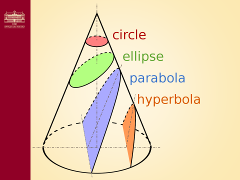
Cones are curves formed at the intersection of two infinitely large cones with a common vertex, an axis and a plane. E.g. a hyperbola occurs when a plane intersects both cones, a circle arises when a plane is perpendicular to the axis of the cone.

Let’s investigate an ellipse.

An ellipse is a plane curve surrounding two focal points (denoted by F1, F2), such that for all points on the curve, the sum of the two distances to the focal points is a constant (|F1P|+|F2P|=const). As such, it generalizes a circle, which is the special type of ellipse in which the two focal points are the same point (F1=F2).

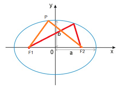
The equation of a standard ellipse centered at the origin with width 2a and height 2b is:

\(\frac{x^{2}}{a^{2}} + \frac{y^{2}}{b^{2}} = 1\)

Assuming a ≥ b, the focal points are (±*c*, 0) for \(c = \sqrt{a^2-b^2}\).

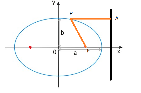
An ellipse may also be defined in terms of one focal point and a line outside the ellipse called the directrix: for all points on the ellipse, the ratio between the distance to the focus and the distance to the directrix is a constant:

• \(e = \frac{c}{a} = (\frac{|PF|}{|PA|})\) numerical eccentricity

To plot ellipses we will use polar coordinates.

In polar coordinates, with the origin at one focus, with the angular coordinate measured from the major axis the ellipse’s equation is

\(r(\theta) = \frac{a(1 - e^{2})}{1 \pm \text{e cos }\theta}\) It could be also writing as

\(r(\theta) = \frac{p}{1 - \varepsilon \bullet cos\theta}\), where

• p is the ordinate of the point above the focus F(c,p)

• \(\varepsilon = \frac{e}{a}\) numerical eccentricity (for ellipse \(\varepsilon < 1\)- for circle \(\varepsilon = 1\) )

Part 1¶

First method-polar coordinate system

Ellipse:

• \(\frac{x^{2}}{25} + \frac{y^{2}}{9} = 1\); a=5, b=3, e=4, p=9/5

\(r(\theta) = \frac{\frac{9}{5}}{1 - \frac{4}{5} \bullet cos\theta}\);\(0{^\circ} \leq \theta < 360{^\circ}\)

Python program for plotting ellipsis

#!/usr/bin/env python3

from ev3dev2.motor import LargeMotor,MediumMotor, OUTPUT_D, OUTPUT_B,OUTPUT_C, SpeedPercent, MoveTank

import math    #v prvih dveh vrsticah naložimo potrebne knjižnice

tank= MoveTank(OUTPUT_B, OUTPUT_C)   #ustvarimo objekt za krmiljenje velikih motorjev B in C

mm=MediumMotor(OUTPUT_D)        #ustvarimo objekt za srednji motor (spust in dvig flumastra)

steps=20   #število točk/korakov

treesixty=2,105  #rotacija potrebna za 360deg

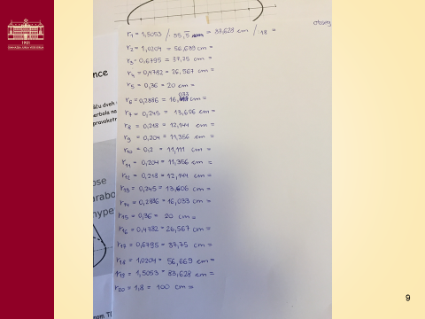
lista=[5.6,3.6,2.3,1.6,1.2,1,0.9,0.85,0.82,0.78,0.78,0.82,0.85,0.9,1,1.2,1.6,2.3,3.6,5.6]   #lista, v kateri so shranjene zračunane razdalje, pretvorjene v število rotacij

for i in range(steps):   #zanko ponovimo 20x

  tank.on_for_rotations(35,35,lista[i])  #se pomakne iz gorišča za razdaljo shranjeno v listi

  mm.on_for_rotations(5,0.15)      #spustimo flumaster

  mm.on_for_rotations(-5,0.15)     #dvignemo flumaster

  tank.on_for_rotations(-35,-35,lista[i])  #se vrne nazaj v gorišče

  tank.on_for_rotations(-5,5,treesixty/steps)  #zarotira za kot (v našem primeru za dvajsetino od 360deg)

Part 2¶

Second method- physical approach

Exercise. Plot a circle with a given radius.

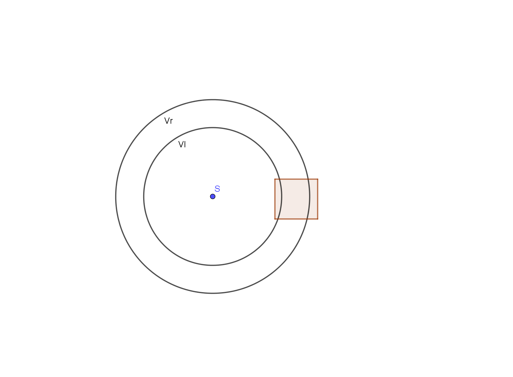
A Circle can be plotted simpler with the help of physics. The left and the right wheels of the robot make different circles at the same time, since the distance between the left and the right wheels is 12 cm. The robot will make a circle with an internal radius of 50 cm in 10 seconds. We will use the following formulas:

\(o_{l} = 2\pi r o_{r} = 2\pi\left( r + 12 \right)\)

\(v = \frac{s}{t}\text{ }v_{l} = \frac{2\pi \bullet 50}{10}\), \(v_{r} = \frac{2\pi \bullet 62}{10}\)

Python program for plotting circle

#!/usr/bin/env python3

from ev3dev2.motor import LargeMotor OUTPUT_D, OUTPUT_B,OUTPUT_C, SpeedPercent, MoveTank

import math    #v prvih dveh vrsticah naložimo potrebne knjižnice

tank= MoveTank(OUTPUT_B, OUTPUT_C)   #ustvarimo objekt za krmiljenje velikih motorjev B in C

v1=30   #hitrost notranjega kolesa

r1=100   #radij notranjega kolesa

r2=r1+12  #radij zunanjega kolesa

v2=v1*r2/r1   #zračunamo hitrost zunanjega kolesa

tank_drive.on(v1,v2)   #poženemo kolesa s hitrostima v1 in v2

|https://ssl.gstatic.com/ui/v1/icons/mail/images/cleardot.gif|

Part 3¶

Ellipse

The parametric ellipse equations are

\(x = a \bullet cost,\ \ y = b \bullet \text{sint}\)

With derivative we get velocities (4th grade)

\(v_{x} = - a \bullet sint,\ \ v_{y} = b \bullet \text{cost.}\)

The total speed on one wheel is

\(v =\sqrt{v_x^2 + v_y^2}\)

We also determine the speed for the outer wheel. The distance between the wheels is 12 cm.