Graph of linear function
The aim of the lesson is to learn the characteristics of the linear function and the way of drawing graphs using robots. There is correlation between mathematics and programming (in Python) . Students are asked to think analytically, using previous knowledge of geometry.
Preparing For This Tutorial
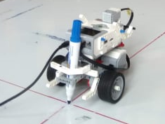
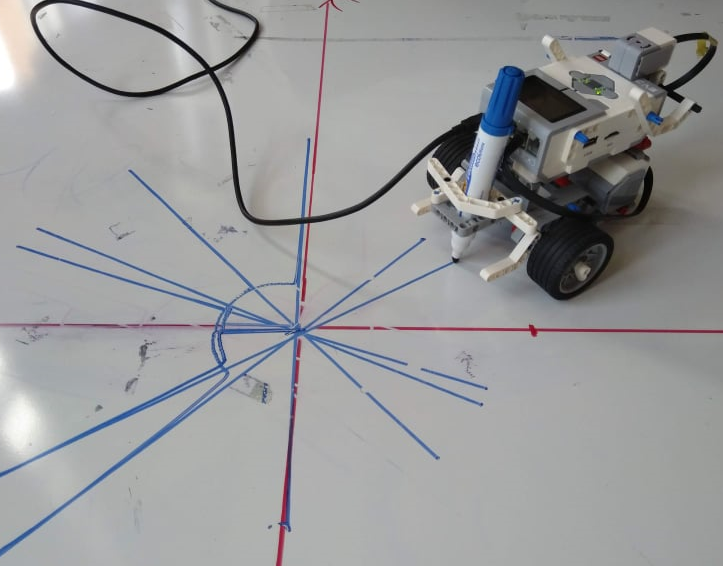
The LEGO Mindstorm EV3 Robot that coincides with this tutorial comes from building specific sections found in the LEGO Mindstorm Education Core Set building instructions. You will need to build the main body for the robot, adapted to draw with some pen, plus gyro sensor and using two servo motors.
Time constraints:
starting from 45 min - single lesson
Exercise
Create a program that will draw a graph of function
f(x)=kx first for k>0 then k<0
f(x)=kx+n for n>0 then n<0
special case when k=0
any kind f(x)=kx+n
Test the program in two ways by making transformations
Vertical shifts f(x)=kx+n
(give k constant ,value k = 1 for the beginning, and change the values for n)
Vertical stretch or compression f(x)=kx+n
(give n constant value,n=0 for the beginning, and change values for k)
Theory
In mathematics there are different kinds of functions.
All of them have special characteristics.
Linear function is the basic.
There are more ways to define it ,and, a more ways of drawing it’s graph
Drawing a graph of a linear function by points
Drawing a graph of a linear function by using y-intercept and slope
(using the segment n, which intersects the line at the у-axis and the angle *α* calculated by the direction coefficient ,through the tangent trigonometric function)
We will use the second way of drawing graphs of linear function by robot.
In the equation f (x) = k x + n
n is the y-intercept of the graph and shows the point (0, n) in which the graph crosses the y-axis.
k is the slope of the line (that is, the incline) is the speed of the change of function, it is also called the coefficient of direction.
The slope of a straight line is given by
k=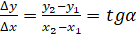
where
α denotes the angle that occupies the graph with the positive part of the x-axis,(x1,y1) and (x2,y2) are two points that belong to the graph (Figure 1).
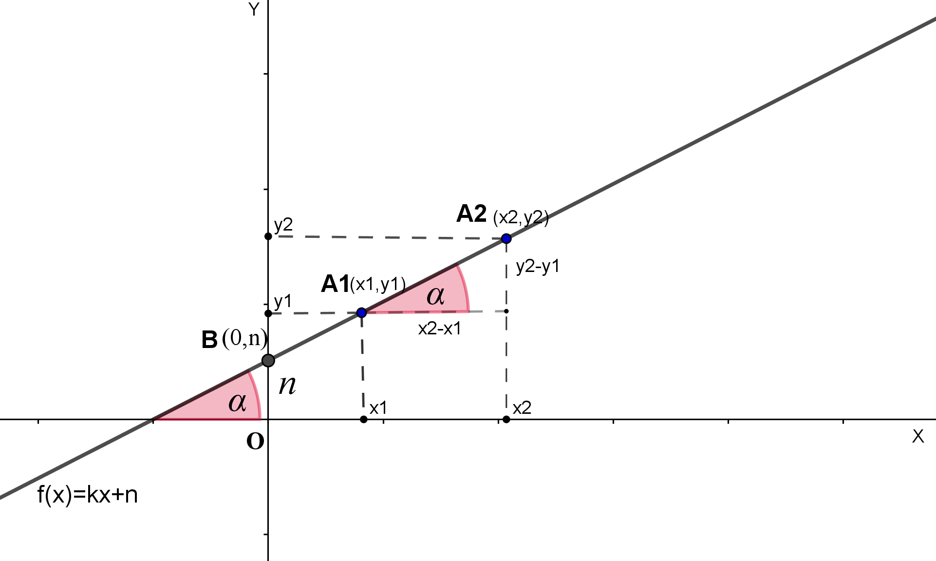
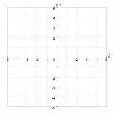
Figure 1.
Graph of linear function
Linear Functions:
Any function of the form f (x) = k x + n, where k is not equal to 0 is called a linear function. The domain of this function is the set of all real numbers. The range of f is the set of all real numbers. The graph of function f is a line with slope k and y- intercept n.
Note: A function f (x) = n, where n is a constant real number is called a constant function. Its graph is a horizontal line parallel with x-axis.
Depending on the value of k, the angle α occupying the graph of the function with the positive direction of the x-axis is determined.
If k>0 then the angle α is less than 90° degrees
If k<0 then the angle is between 90° and 180°
Graphing a Linear Function Using Transformations
Another option for graphing is to use transformations of the identity function f (x)=x . The function can be transformed by moving up, down, left or right.
The function can also be transformed by reflection, stretching, or compression.
Vertical Shift
In f(x)=x+n, the n acts as the vertical shift, moving the graph up and down without affecting the slope of the line. Notice in Figure 2 that adding a value of n to the equation of f(x)=x shifts the graph of f for n units up, if n is positive, and |n| units down if n is negative.
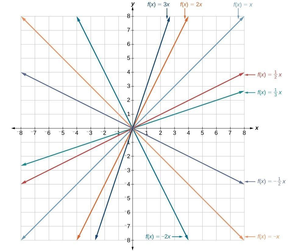
Figure 2.
This graph illustrates vertical shifts of the function f(x)=x.
Vertical Stretch or Compression
In the equation f(x)=kx, the k is acting as the vertical stretch or compression of the identity function. When k is negative, there is also a vertical reflection of the graph. Notice in Figure 3 that multiplying the equation of f(x)=x by k ,stretches the graph of f , if k > 1 , and, compresses the graph of f if 0 < k < 1.
This means the greater the absolute value of k, the greater measure of angle of slope.
Figure 3. Vertical stretches , compressions and reflections on the function f(x)=x.
Python program for drawing linear graph
Commands/functions needed for the exercise
Function: |
Code: |
|---|---|
Connect large motors to port B and C, |
left_motor = LargeMotor(“outB”) right_motor = LargeMotor(“outC”) |
Plug a gyro sensor into any sensor port |
gyro_sensor = GyroSensor() |
Set mode of gyro sensor to work with angles |
gyro_sensor.mode = ‘GYRO-ANG’ |
The function reads a line from input, converts it to a string. If the prompt argument is present, it is written to standard output. In examples: The information that we need is,k & n from y=k*x+n. Also we are pleasing the user to choose the number of drawings that are going to be made. |
input(prompt) Ex: numofAtts=int(input(“Input the number of graphs you want to draw:”)) while(numofAtts>0): k=float(input(“Input k from y=k*x+n:”)) #Input value for k print(“\n”) #New line n=float(input(“Input n from y=k*x+n:”)) #Input value for n |
Depending on the sign and value of n we position the robot on the y axis forward or backward. Note that you can’t put negative value for the time so you need the absolute value of n but setting the motors rotating backwards! Changing the gyro sensor’s mode is a little trick to set the sensor to measure from 0 in the current position and that is why it is easier first to move n and to rotate. |
if(n > 0): #If n is larger than 0 left_motor.run_timed(time_sp=1000*n,speed_sp=100) right_motor.run_timed(time_sp=1000*n,speed_sp=100) if (n < 0): #If n is less than 0 left_motor.run_timed(time_sp=1000*abs(n),speed_sp=-100) right_motor.run_timed(time_sp=1000*abs(n),speed_sp=-100) time.sleep(3) gyro_sensor.mode = ‘GYRO-RATE’ gyro_sensor.mode = ‘GYRO-ANG’ |
Getting the current value which is 0 and we set an integer angle which is also 0 Initially, the angle taken by the robot should be 0, i.e. it is directed along the OY axis |
gcal=abs(gyro_sensor.value()) #Storing value from gyro sensor (-33,33) time.sleep(2) #Rest a bit with functioning angle=0 # |
This is how we compute the angle, it is arctangent from the coefficient k |
angleneeded = abs(math.degrees(math.atan(k))) |
As the comments say, this is the process for setting up the complementary angle that the graph has with the axis y since we are moving from y-axis to the left or to the right.Angle is constantly updating on every rotation that the robot makes and if the difference between the starting position and current angle is complementary then we have the desired angle and we are prepared for the next step which is – drawing the line. |
if k<0: #If k is less than 0 then the angle is > 90 while abs(angle-gcal)<90-angleneeded: #While we don’t achieve the needed complementary angle left_motor.run_forever(speed_sp=-10) #Move the robot to the right_motor.run_forever(speed_sp=10) #Right angle=abs(gyro_sensor.value()) #Constantly update the angle print(angle) print(gcal) elif k >= 0: #If k is large than 0 then the angle is < 90 gcal=abs(gyro_sensor.value()) angle=abs(gyro_sensor.value()) #if gyro_sensor.value()<0: # angleneeded+=abs(gyro_sensor.value()) while angle-gcal<abs(90-angleneeded): #While we don’t achieve the needed complementary angle left_motor.run_forever(speed_sp=10) #Move the robot to the right_motor.run_forever(speed_sp=-10) #Left angle=abs(gyro_sensor.value()) |
Now we want to be sure that the motors are stopped,and we move the robot to some point backwards so we can get some idea of what is the direction forward.Then we are moving the robot forward so we can have the idea what the graph looks like below the intersection point. We reduce the number of attempts since we have finished drawing (plot). raise SystemExit is the call that we use to interrupt the program(note that is outside the loop and theat we need to stop the program after the number of attempts is equal to zero. The SystemExit raise is called to interrupt the program (note that it is outside the loop and we need to stop the program when the number of attempts is zero). |
#Assuring that we didn’t made motors to move @ all left_motor.stop() #When we get out from the loop right_motor.stop()# we make the robot to stop rotating since it achieved the desired angle left_motor.run_timed(time_sp=3250,speed_sp=100,stop_action=”brake”) #Moving the robot to some point backwards *Both motors right_motor.run_timed(time_sp=3250,speed_sp=100,stop_action=”brake”) #Moving the robot to some point backwards *Both motors time.sleep(8) #The robot is tired,and calculates ;) left_motor.run_timed(time_sp=6500,speed_sp=-100,stop_action=”brake”) #Moving the robot to some point backwards *Both motors right_motor.run_timed(time_sp=6500,speed_sp=-100,stop_action=”brake”) #Moving the robot to some point backwards *Both motors time.sleep(5) numofAtts-=1
raise SystemExit
|
Name and surname _______________ Date _____
Graph of linear function
Worksheet for students
Draw a graph of a linear function
а) f(x)=kx for k>0 , k<0
f(x)=kx+n for n>0 , n<0
special case k =0
any kind f(x)=kx+n
In the drawings, mark the angles that occupy the graph with the x-axis and calculate their sizes.
а)
 б)
б)
b)
г)
Create a program that will draw a graph of function
f(x)=kx
f(x)=kx+n
f(x)=n special case k =0
Test the program by making transformations in two ways:
Vertical shifts
f(x)=kx+n (give k for a constant value, change the values for n)
Vertical stretch or compression
f(x)=kx+n (give n for a constant value, change the values for k)
Draw the graphs of the functions that are obtained with the corresponding transformations.
- ( k-constant, n-variable)
- ( n-constant, k-variable)