Acceleration Due to Gravity with Lego EV3 & Python
Aim of the lesson
Welcome to the lesson on Gravitational Acceleration!
The aim of the lesson is to research experientially topics related to the gravitational acceleration g, learned theoretically during physics class, and try to answer questions that arise, such as what about g for different heights or for heavier/lighter objects. You will execute an experiment that involves the construction of a Lego EV3 drop tower equipped with suitable sensors and programmed in Python language for calculating g affecting a ball in free fall. In the process of experiment you’ll have to remember and apply mathematics notions, such as that of slope.
We would like to show you that Robotics can be very helpful when used to collect data in physics experiments, giving you the motivation to try Robotics to other physics concepts, as well. Robotics for measuring g can provide an accurate and reliable result. Times less than 1 secs are difficult to measure with a conventional clock. Synchronization of leaving a ball and thereby counting falling time is extremely difficult to obtain.
Preparing For This Tutorial:
First Steps:
The LEGO Mindstorm EV3 Robot that coincides with this experiment comes from building specific sections found in the LEGO Mindstorm Education Core Set building instructions and it is attached here as a pdf file in the building_instructions folder. You will need to build the robot and if you want you may replace the touch sensor with a color sensor for better results.
You can also build another model of robot for g using the attached measuring_g_building_instructions ldd/html file. It’s another flexible model for calculating g with larger balls and using touch sensors.
Next Steps:
Load the EV3 brick with a readymade EV3-dev SD card, which your teacher will give to you.
Set up the network connection between the EV3 and the brick, as described
Set up a graphical SSH connection between the EV3 and the PC, as described
Establish a WiFi connection between the EV3 and the PC. (Instructions can be found here http://sites.google.com/site/ev3python/wireless/wifi-connectivity )
Exercise
Implement a distributed python program (PC/EV3)
Sensor and motor control is performed on EV3
The computation and graph section for g runs on the PC.
What does a Python program have to do?
It commands the motor to release the object from the claw
Once it hits on the touch / color sensor it counts the down time
Calculates the speed in relation to time for different release heights
Designs a speed / time graph on the computer screen
Calculates and displays the gradient of this graph (it’s the half of experimental value of g)
Compare experimental value of g to the standard value of g (9.81 m/sec2)
Compare the values for the measured acceleration of the different objects and different heights tested.
What are the possible explanations for the difference in the values for your measured g and the accepted value of g?
Time constraints:
3-4 hrs
Theory
The concepts of Physics are apparent in all areas of our world. A fundamental understanding of the role of gravity is the foundation for many feats of engineering that we see in our everyday lives, such as bridges, buildings, airplanes, etc. Gravity is commonly thought of as a universal force that holds matter together. It results from the net force the Earth exerts on objects in its vicinity. On the surface, gravity is the net force that is responsible for downward motion of free falling objects. It accelerates all objects at the same rate.
Newton’s second law states that the net force on an object is equal to the mass of the object times its acceleration;
F = ma (1)
where m is mass and a is acceleration. For an object in free fall, equation one can be written as;
F = mg (2)
where m is mass and g is the acceleration due to gravity. Equating equations 1 and 2 shows that the acceleration of the object is due to force of gravity and is independent of mass;
F = ma = mg 🡪 a= g (3)
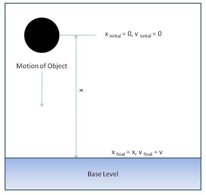
For a conservative system, the total amount of energy remains constant. In our setup, only forces in the vertical direction come into play (neglect air resistance). At the beginning of the experiment, the object is fixed at a specified distance above some base level (e.g. the ground). At the starting position, the object is considered to have potential energy (PE) but no kinetic energy (KE). As soon as the object is released, some of its PE is converted to KE, and the object begins to fall (due to gravity). As freefall continues more of its PE is converted to KE and the velocity of the object increases. This change in the object’s velocity as it falls is the acceleration due to gravity, g, which has a constant value of 9.8 m/s2.
If we only look at the downward motion of the object (one dimension), its acceleration, g, is defined as the rate of change of its velocity with respect to time. Mathematically, the acceleration is derivative of velocity with respect to time, such that;
g = dv / dt
Assuming that the object accelerates from some initial velocity, v0 to some final velocity, vf, over a time interval of t0 to t, then applying these conditions to the integration of equation (1) yields the final velocity of the object:
vf = v0 + gt
Velocity is defined as the change of an object’s position with respect to time;
v = dx / dt
Assuming that the object travels from some initial position, x0 to a final one, x, over the same time interval as before (t:sub:0,t), an equation for position can be derived. Combining equations (2) and (3) and integrating over the conditions of x0 to x, and t0 to t, the position of the object is;
x = x0 + v0t + ½ gt2
We will be measuring the average velocity, such that:
vavg = ½ (v:sub:f + v0)
where vf and vo are the final and initial velocities, respectively. Substitution of equation 5 into equation 2 yields:
vavg = v0 + ½ gt
Vocabulary / Definitions
Word |
Definition |
|---|---|
Potential Energy |
The energy of position |
Kinetic energy |
The energy of motion |
Gravity |
the force of attraction by which terrestrial bodies tend to fall toward the center of the earth |
Velocity |
The rate of change of position with respect to time. |
Acceleration |
The rate of change of velocity with respect to time. |
You can also watch the following interactive videos at home from the *Edpuzzle *site (First create a student account on this platform with your details and join the PROBOT class with code that your teacher will give you). As you watch each video, you will answer relevant questions that are embedded in appropriate points in the video.
Introduction to Free-Fall and the Acceleration due to Gravity (Interactive video)
Acceleration Due to Gravity tutorial (interactive video)
The Acceleration due to Gravity (interactive video)
Calculating Acceleration Due to Gravity (g) (interactive video)
Short help on programming
Commands/functions needed for the exercise
Connect large motor to port B |
b = ev3.LargeMotor(‘outB’) |
Run to a position relative to the current position value. The new position will be current position + position_sp. This works because the motors are “smart” and have a sensor that can detect the number of degrees the motor has turned. When the new position is reached, the motor will stop using the action specified by stop_action. On the example one rotation of wheels |
run_to_rel_pos(position_sp=<angle in degrees>, speed_sp=<value>,stop_action=<value>) speed_sp is between 0 and 1000 position_sp >0 Motor will run forward position_sp <0 Motor will run backwards stop_action - can be “coast”or “brake” or “hold” b.run_to_rel_pos(position_sp=360, speed_sp=200,stop_action= “brake “) |
Turn motor for an unspecified time i.e. until another command is sent. |
run_forever(speed_sp=<value>) b.runforever(speed_sp=90) |
Stop the motor |
stop() stop(stop_action=<value>) where <value> can be “coast”, “brake” or “hold”. |
Plug a touch sensor into any sensor port |
touch = ev3.TouchSensor() Here touch is the name we choose to use for the sensor. You can use any name you wish. This command will search the ports for a Touch Sensor and save its location if it finds one. You will get an error if it doesn’t find one. |
Reading the Touch Sensor |
touch.value() This function will return a numeric value. Since this is a touch sensor, there are only two possible values: 0 tells you the button is not currently pushed, 1 tells you the button is pushed. You could have the Touch Sensor and Large Motor interact using the following simple program. from ev3 import * m = LargeMotor() t = TouchSensor() m.run_forever(speed_sp=500) while (t.value() == 0): pass m.stop() t will run the motor until the sensor is pressed. |
Plug a color sensor into any sensor port |
color = ColorSensor() Here color is the name we choose to use for the sensor. You can use any name you wish. This command will search the ports for a Color Sensor and save its location if it finds one. You will get an error if it doesn’t find one. |
Set mode of color sensor |
This sensor has several modes. It can detect reflected light intensity (‘COL-REFLECT’), ambient light intensity (‘COL-AMBIENT’), and color (‘COL-COLOR’). You set the mode by setting the mode parameter. For example to detect ambient light intensity you could do the following: color = ColorSensor() color.mode = ‘COL-AMBIENT’ |
Reading the Color Sensor |
color.value() For example to detect ambient light intensity you could do the following: color = ColorSensor() color.mode = ‘COL-AMBIENT’ color.value() This would return the current ambient light intensity as a number between 0 and 100 where 0 is complete darkness. The process for measuring reflected light is the same except the mode is set to ‘COL-REFLECT’. The color mode is a little different. If you set the mode to ‘COL-COLOR’ then the return value will be an integer in the range 0-7. The values are as follows
The following program would run the Large Motor until the Color Sensor sees red. from ev3 import * m = LargeMotor() c = ColorSensor() c.mode = ‘COL-COLOR’ m.run_forever(speed_sp=500) while (c.value() != 5): pass m.stop() |
polyfit(x, y, deg, rcond=None, full=False, w=None) |
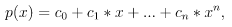
Least-squares fit of a polynomial to data. Return the coefficients of a polynomial of degree deg that is the least squares fit to the data values y given at points x. If y is 1-D the returned coefficients will also be 1-D. If y is 2-D multiple fits are done, one for each column of y, and the resulting coefficients are stored in the corresponding columns of a 2-D return. The fitted polynomial(s) are in the form
where n is deg. Example: >>> y = x\*\*3 - x
>>> c, stats = P.polyfit(x,y,3,full=True)
>>> c # c[0], c[2] should be "very close to 0", c[1] ~= -1, c[3] ~= 1
array([ -1.73362882e-17, -1.00000000e+00, -2.67471909e-16, 1.00000000e+00]) |
plot() is a versatile command, and will take an arbitrary number of arguments. For example, to plot x versus y, you can issue the command: plot([1, 2, 3, 4], [1, 4, 9, 16]) For every x, y pair of arguments, there is an optional third argument which is the format string that indicates the color and line type of the plot. The letters and symbols of the format string are from MATLAB, and you concatenate a color string with a line style string. The default format string is ‘b-‘, which is a solid blue line. For example, to plot the above with red circles, you would issue import matplotlib.pyplot as plt plt.plot([1,2,3,4], [1,4,9,16], ‘ro’) plt.axis([0, 6, 0, 20]) plt.show() |
|
The axis() command takes a list of [xmin, xmax, ymin, ymax] and specifies the viewport of the axes. |
Working with ev3dev remotely using RPyC (Distributed programming)
RPyC(pronounced as are-pie-see), or Remote Python Call, is a transparent python library for symmetrical remote procedure calls, clustering and distributed-computing. RPyC makes use of object-proxying, a technique that employs python’s dynamic nature, to overcome the physical boundaries between processes and computers, so that remote objects can be manipulated as if they were local. Here are simple steps you need to follow in order to install and use RPyC with ev3dev:
Install RPyC both on the EV3 and on your desktop PC. For the EV3, enter the following command at the command prompt (after you connect with SSH):
On the desktop PC, it really depends on your operating system. In case it is some flavor of linux, you should be able to do
In case it is Windows, there is a win32 installer on the project’s sourceforge page. Also, have a look at the Download and Install page on their site.
Create file rpyc_server.sh with the following contents on the EV3:
and make the file executable:
Launch the created file either from SSH session (with ./rpyc_server.sh command), or from brickman. It should output something like
and keep running.
Now you are ready to connect to the RPyC server from your desktop PC. The following python script should make a large motor connected to output port A spin for a second.
You can run scripts like this from any interactive python environment, like ipython shell/notebook, spyder, pycharm, etc.
Some advantages of using RPyC with ev3dev are:
It uses much less resources than running an ipython notebook on EV3; RPyC server is lightweight, and only requires an IP connection to the EV3 once set up (no ssh required).
The scripts you are working with are actually stored and edited on your desktop PC, with your favorite editor/IDE.
Some robots may need much more computational power than what EV3 can give you. A notable example is the Rubik’s cube solver: there is an algorithm that provides an almost optimal solution (in terms of number of cube rotations), but it takes more RAM than is available on EV3. With RPYC, you could run the heavy-duty computations on your desktop.
The most obvious disadvantage is latency introduced by network connection. This may be a show stopper for robots where reaction speed is essential.
External modules - rpyc, time, pylab